The Penguin Dataset

Below is the Palmer Penguins data set collected by Dr. Kristen Gorman and the Palmer Station, Antarctica LTER. The data contains physiological measurements for a number of penguins from each of three species of penguin: Chinstrap, Gentoo, and Adelie.

Code

import pandas as pd
import numpy as np
from matplotlib import pyplot as plt

train_url = "https://raw.githubusercontent.com/middlebury-csci-0451/CSCI-0451/main/data/palmer-penguins/train.csv"
train = pd.read_csv(train_url)
train.head()

	studyName	Sample Number	Species	Region	Island	Stage	Individual ID	Clutch Completion	Date Egg	Culmen Length (mm)	Culmen Depth (mm)	Flipper Length (mm)	Body Mass (g)	Sex	Delta 15 N (o/oo)	Delta 13 C (o/oo)	Comments
0	PAL0708	27	Gentoo penguin (Pygoscelis papua)	Anvers	Biscoe	Adult, 1 Egg Stage	N46A1	Yes	11/29/07	44.5	14.3	216.0	4100.0	NaN	7.96621	-25.69327	NaN
1	PAL0708	22	Gentoo penguin (Pygoscelis papua)	Anvers	Biscoe	Adult, 1 Egg Stage	N41A2	Yes	11/27/07	45.1	14.5	215.0	5000.0	FEMALE	7.63220	-25.46569	NaN
2	PAL0910	124	Adelie Penguin (Pygoscelis adeliae)	Anvers	Torgersen	Adult, 1 Egg Stage	N67A2	Yes	11/16/09	41.4	18.5	202.0	3875.0	MALE	9.59462	-25.42621	NaN
3	PAL0910	146	Adelie Penguin (Pygoscelis adeliae)	Anvers	Dream	Adult, 1 Egg Stage	N82A2	Yes	11/16/09	39.0	18.7	185.0	3650.0	MALE	9.22033	-26.03442	NaN
4	PAL0708	24	Chinstrap penguin (Pygoscelis antarctica)	Anvers	Dream	Adult, 1 Egg Stage	N85A2	No	11/28/07	50.6	19.4	193.0	3800.0	MALE	9.28153	-24.97134	NaN

Preparing our dataset

Our data frame has some columns we can’t use directly. Thus, we used the “one-hot encoding” to represent these features as binary columns.

Code

from sklearn.preprocessing import LabelEncoder
le = LabelEncoder()
le.fit(train["Species"])

def prepare_data(df):
  df = df.drop(["studyName", "Sample Number", "Individual ID", "Date Egg", "Comments", "Region"], axis = 1)
  df = df[df["Sex"] != "."]
  df = df.dropna()
  y = le.transform(df["Species"])
  df = df.drop(["Species"], axis = 1)
  df = pd.get_dummies(df)
  return df, y

X_train, y_train = prepare_data(train)

Code

X_train.head()

	Culmen Length (mm)	Culmen Depth (mm)	Flipper Length (mm)	Body Mass (g)	Delta 15 N (o/oo)	Delta 13 C (o/oo)	Island_Biscoe	Island_Dream	Island_Torgersen	Stage_Adult, 1 Egg Stage	Clutch Completion_No	Clutch Completion_Yes	Sex_FEMALE	Sex_MALE
1	45.1	14.5	215.0	5000.0	7.63220	-25.46569	1	0	0	1	0	1	1	0
2	41.4	18.5	202.0	3875.0	9.59462	-25.42621	0	0	1	1	0	1	0	1
3	39.0	18.7	185.0	3650.0	9.22033	-26.03442	0	1	0	1	0	1	0	1
4	50.6	19.4	193.0	3800.0	9.28153	-24.97134	0	1	0	1	1	0	0	1
5	33.1	16.1	178.0	2900.0	9.04218	-26.15775	0	1	0	1	0	1	1	0

Looking at body mass and sex in the 3 species

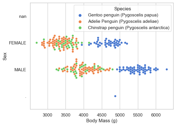
The displayed figure below shows the general relationship between sex and body mass (g) in each of the 3 penguin species. By looking at the figure, it’s clear that female penguins tend to have a lower body mass than the male penguins. In addition, the Gentoo penguins have a larger overall body mass than the other 2 species, weighing between 4000 to 6000 grams. Both the Adelie and Chinstap species weigh between 3000 to 4500 grams.

Code

import seaborn as sns
sns.set_theme(style="whitegrid", palette="muted")

# Draw a categorical scatterplot to show each observation
ax = sns.swarmplot(data=train, x="Body Mass (g)", y="Sex", hue="Species")
ylab = ax.set(ylabel="Sex")

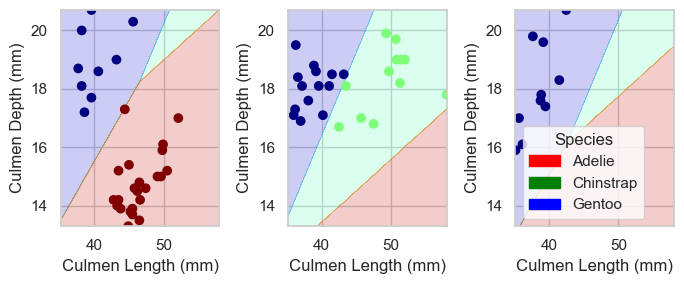
Comparing flipper lengths of the 3 species

The table below shows clear differences in flipper lengths between the 3 species. Gentoo penguins have the largest overall flipper length at 217.65mm. The Chinstrap penguins’ overall flipper length comes in at 195.46mm. Adelie penguins have the smallest overall flipper length of the 3 species, at 189.97mm. However, it’s important to note that there was much less data recorded for the Chinstrap species as compared to the other 2 species.

Code

train.groupby(['Species'])[['Flipper Length (mm)']].aggregate([np.mean,len ]).round(2)

	Flipper Length (mm)
	mean	len
Species
Adelie Penguin (Pygoscelis adeliae)	189.97	118
Chinstrap penguin (Pygoscelis antarctica)	195.46	56
Gentoo penguin (Pygoscelis papua)	217.65	101

Modeling

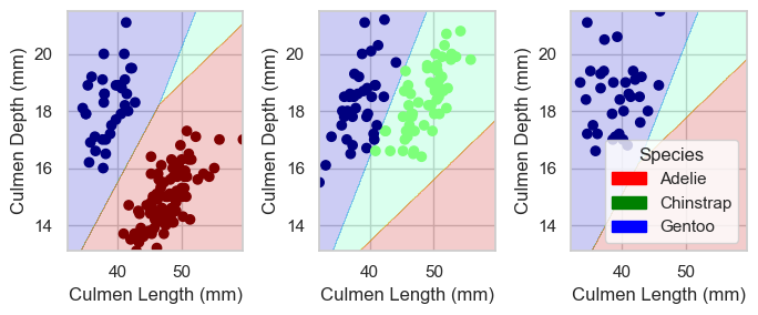
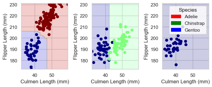
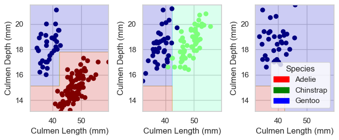
Below, we perform an exhaustive search of all the features contained in the dataset to find the 3 best features that will achieve 100% accuracy. The models that we will implement are Logistic Regression, Random Forest Classifier and Decision Tree Classifier, all of which are taken from sklearn.

Code

from itertools import combinations
from sklearn.linear_model import LogisticRegression
from sklearn.ensemble import RandomForestClassifier
from sklearn.tree import DecisionTreeClassifier

import warnings

warnings.filterwarnings("ignore")

all_qual_cols = ["Clutch Completion", "Sex", "Island"]
all_quant_cols = ['Culmen Length (mm)', 'Culmen Depth (mm)', 'Flipper Length (mm)', 'Body Mass (g)']

best_score_LR = 0              #highest accuracy reached with LR model
best_score_RF = 0              #highest accuracy reached with RF model
best_score_DT = 0              #highest accuracy reached with DT model

for qual in all_qual_cols: 
  qual_cols = [col for col in X_train.columns if qual in col ]
  for pair in combinations(all_quant_cols, 2):
    cols = list(pair) + qual_cols 
    
    #  train on logistic regression
    LR = LogisticRegression()
    LR.fit(X_train[cols], y_train)

    # keeping the list of columns for the model that has the best score 
    if (LR.score(X_train[cols], y_train) > best_score_LR):
       best_cols_LR = cols
       best_score_LR = LR.score(X_train[cols], y_train)
       best_LR = LR

    # train on random forest classifier
    RF = RandomForestClassifier(max_depth=3, random_state=0)
    RF.fit(X_train[cols], y_train)

    # keeping the list of columns for the model that has the best score 
    if (RF.score(X_train[cols], y_train) > best_score_RF):
       best_cols_RF = cols
       best_score_RF = RF.score(X_train[cols], y_train)
       best_RF = RF

   # train on decision tree classifier
    DT = DecisionTreeClassifier(max_depth=3)
    DT.fit(X_train[cols], y_train)

    # keeping the list of columns for the model that has the best score 
    if (DT.score(X_train[cols], y_train) > best_score_DT):
       best_cols_DT = cols
       best_score_DT = DT.score(X_train[cols], y_train)
       best_DT = DT

print("Best 3 columns for LR: " + str(best_cols_LR))
print("Training Accuracy for LR: " + str(best_score_LR))

print("\nBest 3 columns for RF: " + str(best_cols_RF))
print("Training Accuracy for RF: " + str(best_score_RF))

print("\nBest 3 columns for DT: " + str(best_cols_DT))
print("Training Accuracy for DT: " + str(best_score_DT))

Best 3 columns for LR: ['Culmen Length (mm)', 'Culmen Depth (mm)', 'Island_Biscoe', 'Island_Dream', 'Island_Torgersen']
Training Accuracy for LR: 1.0

Best 3 columns for RF: ['Culmen Length (mm)', 'Flipper Length (mm)', 'Island_Biscoe', 'Island_Dream', 'Island_Torgersen']
Training Accuracy for RF: 0.9921875

Best 3 columns for DT: ['Culmen Length (mm)', 'Culmen Depth (mm)', 'Island_Biscoe', 'Island_Dream', 'Island_Torgersen']
Training Accuracy for DT: 0.9921875

Cross-Validation

We will use cross-validation to get a sense for what max depth we should set for the Decision Tree Classifier.

Code

from sklearn.model_selection import cross_val_score

cv_scores = cross_val_score(best_DT, X_train[best_cols_DT], y_train, cv=5)
cv_scores

array([1.        , 0.94117647, 0.98039216, 0.98039216, 0.98039216])

Code

max_depth = 5

while max_depth != 0:
  DT = DecisionTreeClassifier(max_depth = max_depth)
  cv_scores = cross_val_score(DT, X_train[best_cols_DT], y_train, cv=5)
  mean_score = cv_scores.mean()
  print(f"Max depth = {max_depth}, score = {mean_score.round(3)}")
  max_depth += -1

Max depth = 5, score = 0.98
Max depth = 4, score = 0.98
Max depth = 3, score = 0.976
Max depth = 2, score = 0.945
Max depth = 1, score = 0.731

Plotting Decision Regions

Code

from matplotlib.patches import Patch

warnings.filterwarnings("ignore")

def plot_regions(model, X, y):
    
    x0 = X[X.columns[0]]
    x1 = X[X.columns[1]]
    qual_features = X.columns[2:]
    
    fig, axarr = plt.subplots(1, len(qual_features), figsize = (7, 3))

    # create a grid
    grid_x = np.linspace(x0.min(),x0.max(),501)
    grid_y = np.linspace(x1.min(),x1.max(),501)
    xx, yy = np.meshgrid(grid_x, grid_y)
    
    
    XX = xx.ravel()
    YY = yy.ravel()

    for i in range(len(qual_features)):
      XY = pd.DataFrame({
          X.columns[0] : XX,
          X.columns[1] : YY
      })

      for j in qual_features:
        XY[j] = 0

      XY[qual_features[i]] = 1

      p = model.predict(XY)
      p = p.reshape(xx.shape)
      
      
      # use contour plot to visualize the predictions
      axarr[i].contourf(xx, yy, p, cmap = "jet", alpha = 0.2, vmin = 0, vmax = 2)
      
      ix = X[qual_features[i]] == 1
      # plot the data
      axarr[i].scatter(x0[ix], x1[ix], c = y[ix], cmap = "jet", vmin = 0, vmax = 2)
      
      axarr[i].set(xlabel = X.columns[0], 
            ylabel  = X.columns[1])
      
      patches = []
      for color, spec in zip(["red", "green", "blue"], ["Adelie", "Chinstrap", "Gentoo"]):
        patches.append(Patch(color = color, label = spec))

      plt.legend(title = "Species", handles = patches, loc = "best")
      
      plt.tight_layout()

Plotting decision regions for the Logistic Regression model on its 3 best chosen features: culmen length, culmen depth, and island.

Code

plot_regions(best_LR, X_train[best_cols_LR], y_train)

Plotting decision regions for the Random Forest classifier on its 3 best chosen features: culmen length, flipper length, and island.

Code

plot_regions(best_RF, X_train[best_cols_RF], y_train)

Plotting decision regions for the Decision Tree classifier on its 3 best chosen features: culmen length, flipper length, and island.

Code

plot_regions(best_DT, X_train[best_cols_DT], y_train)

Testing

Since the Logistic Regression model yields the highest accuracy, we will use that on our test data.

Code

test_url = "https://raw.githubusercontent.com/middlebury-csci-0451/CSCI-0451/main/data/palmer-penguins/test.csv"
test = pd.read_csv(test_url)

X_test, y_test = prepare_data(test)

print ("Testing accuracy for Logistic Regression: " + str(best_LR.score(X_test[best_cols_LR], y_test)))

Testing accuracy for Logistic Regression: 1.0

Code

plot_regions(best_LR, X_test[best_cols_LR], y_test)
plt.savefig("image.jpg")