The Data

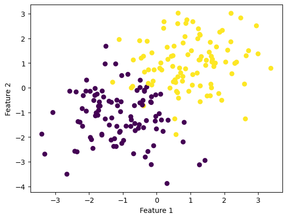
Below is a nonseparable data in which we will apply the gradient descent and stochastic gradient descent methods on.

Code

from sklearn.datasets import make_blobs
from matplotlib import pyplot as plt
import numpy as np
np.seterr(all='ignore') 

# making the data
p_features = 3
X, y = make_blobs(n_samples = 200, n_features = p_features - 1, centers = [(-1, -1), (1, 1)])

fig = plt.scatter(X[:,0], X[:,1], c = y)
xlab = plt.xlabel("Feature 1")
ylab = plt.ylabel("Feature 2")

Regular Gradient Descent

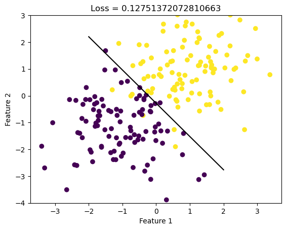
We will use gradient descent to compute a value of the parameter vector \(\tilde{w}\). Here, convergence for gradient descent is declared when the improvement in the function is small enough in magnitude. Fit() utilizes the following function to obtain the gradient of the empirical risk for logistic regression:

\[\nabla L(w) = \frac{1}{n}\sum_{i = 1}^n \nabla \ell(f_{w}(x_i), y_i)\;\]

Then, we can do logistic regression by choosing a learning rate and iterating the update \(\mathbf{w}^{(t+1)} \gets \mathbf{w}^{(t)} - \alpha \nabla L(\mathbf{w}^{(t)})\) until convergence.

Code

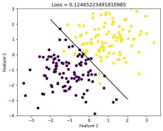
from LogisticRegression import LogisticRegression

LR = LogisticRegression()
LR.fit(X, y, 0.1, 1000)

def draw_line(w, x_min, x_max):
  x = np.linspace(x_min, x_max, 101)
  y = -(w[0]*x + w[2])/w[1]
  plt.plot(x, y, color = "black")

fig = plt.scatter(X[:,0], X[:,1], c = y)
fig = draw_line(LR.w, -2, 2)
plt.ylim(-4,3)

xlab = plt.xlabel("Feature 1")
ylab = plt.ylabel("Feature 2")

loss = LR.loss(X, y)
title = plt.title(f"Loss = {loss}")

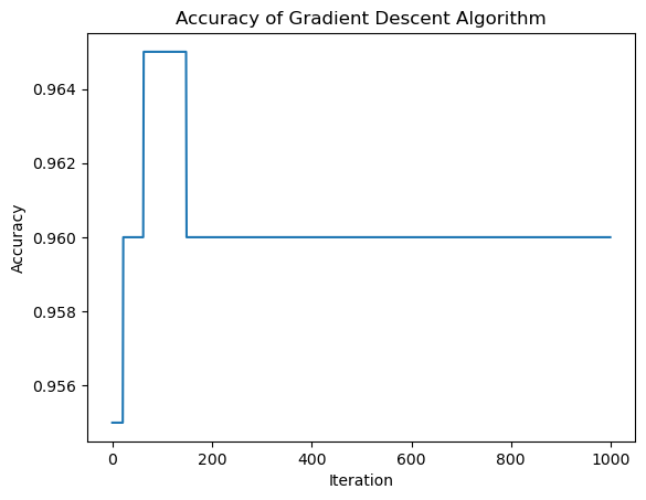
Accuracy of Regular Gradient Descent

Code

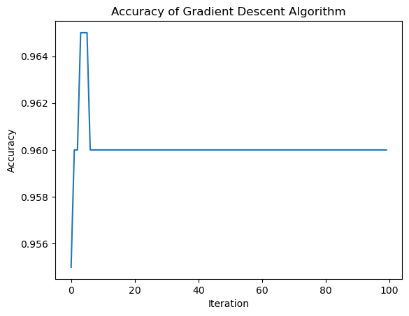
print("Evolution of the score over the training period (last few scores):") 
print(LR.score_history[-10:]) #just the last few scores

fig = plt.plot(LR.score_history)
xlab = plt.xlabel("Iteration")
ylab = plt.ylabel("Accuracy")
title = plt.title("Accuracy of Gradient Descent Algorithm")

Evolution of the score over the training period (last few scores):
[0.96, 0.96, 0.96, 0.96, 0.96, 0.96, 0.96, 0.96, 0.96, 0.96]

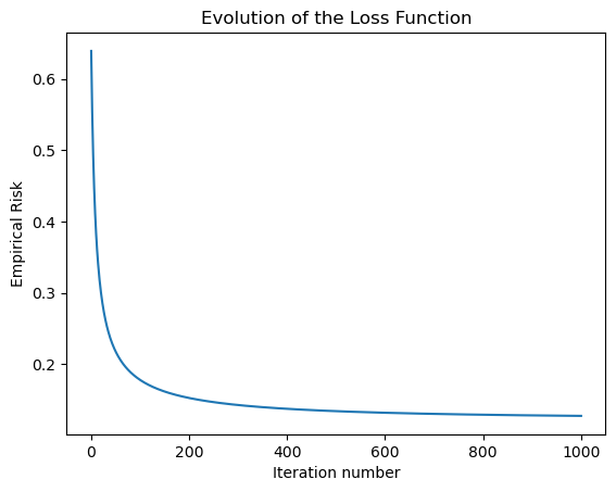
Empirical Risk of Regular Gradient Descent

Code

print("Evolution of the loss over the training period (last few losses):") 
print(LR.loss_history[-10:]) #just the last few losses

fig = plt.plot(LR.loss_history)
xlab = plt.xlabel("Iteration number")
ylab = plt.ylabel("Empirical Risk")
title = plt.title("Evolution of the Loss Function")

Evolution of the loss over the training period (last few losses):
[0.12756465548793788, 0.12755823771168123, 0.12755183457409008, 0.1275454460315202, 0.12753907204049475, 0.12753271255770313, 0.12752636754000055, 0.127520036944407, 0.12751372072810663, 0.12751372072810663]

Stochastic Gradient Descent

In stochastic gradient descent, we pick a random subset \(S \subseteq [n] = \{1, \ldots, n\}\) and compute:

\[\nabla_S L(w) = \frac{1}{{|S|}}\sum_{i \in S} \nabla \ell(f_{w}(x_i), y_i)\;\]

Again, convergence is declared when the improvement in the function is small enough in magnitude.

Code

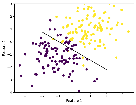
LR = LogisticRegression()
LR.fit_stochastic(X, y, 0.1, 100, 10)

fig = plt.scatter(X[:,0], X[:,1], c = y)
fig = draw_line(LR.w, -2, 2)
plt.ylim(-4,3)

xlab = plt.xlabel("Feature 1")
ylab = plt.ylabel("Feature 2")

loss = LR.loss(X, y)
title = plt.title(f"Loss = {loss}")

Accuracy of Stochastic Gradient Descent

Code

print("Evolution of the score over the training period:") 
print(LR.score_history[-10:]) #just the last few scores

fig = plt.plot(LR.score_history)
xlab = plt.xlabel("Iteration")
ylab = plt.ylabel("Accuracy")
title = plt.title("Accuracy of Gradient Descent Algorithm")

Evolution of the score over the training period:
[0.96, 0.96, 0.96, 0.96, 0.96, 0.96, 0.96, 0.96, 0.96, 0.96]

Empirical Risk of Stochastic Gradient Descent

Code

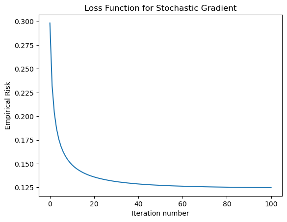
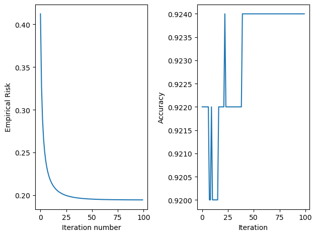
print("Evolution of the loss over the training period:") 
print(LR.loss_history[-10:]) #just the last few scores

fig = plt.plot(LR.loss_history)
xlab = plt.xlabel("Iteration number")
ylab = plt.ylabel("Empirical Risk")
title = plt.title("Loss Function for Stochastic Gradient")

Evolution of the loss over the training period:
[0.12482870714265093, 0.1248063720546357, 0.12478314821058926, 0.1247593290029095, 0.12473696450872014, 0.12471412006229605, 0.1246933964041914, 0.12467358666704516, 0.12465223491810985, 0.12465223491810985]

Nonconvergence in Gradient Descent

Below is an illustration in which gradient descent does not converge to a minimizer because the learning rate \(\alpha\) is too large.

Code

LR = LogisticRegression()
LR.fit(X, y, 500, 1000)

def draw_line(w, x_min, x_max):
  x = np.linspace(x_min, x_max, 101)
  y = -(w[0]*x + w[2])/w[1]
  plt.plot(x, y, color = "black")

fig = plt.scatter(X[:,0], X[:,1], c = y)
fig = draw_line(LR.w, -2, 2)
plt.ylim(-4,3)

xlab = plt.xlabel("Feature 1")
ylab = plt.ylabel("Feature 2")

Choice of Batch Size in Stochastic Gradient Descent

Below is an illustration in which the choice of batch size influences how quickly the algorithm converges.

Code

p_features = 11
X, y = make_blobs(n_samples = 500, n_features = p_features - 1, centers = [(-1, -1), (1, 1)])

LR = LogisticRegression()
LR.fit_stochastic(X, y, 0.1, 100, 50)

fig, axarr = plt.subplots(1, 2)

fig = axarr[0].plot(LR.loss_history)
axarr[0].set(xlabel = "Iteration number", ylabel = "Empirical Risk")

fig = axarr[1].plot(LR.score_history)
axarr[1].set(xlabel = "Iteration", ylabel = "Accuracy")

plt.tight_layout()
plt.savefig("image.jpg")